
Biology for Data Scientists: Understanding the Genetic Pipeline
So, you’re a data scientist trying to make your way into bioinformatics. There’s plenty of data to analyze, and your knowledge of algorithms, models, and methods will surely give you a head start…
But first, you need to brush up on some high school biology and level up fast. Because there’s a lot, and I mean a lot, of jargon in this field. The data structures themselves aren’t necessarily complicated (though they can get pretty deep), but the terminology is another story. You need to know what all those pesky terms are referring to.
Sure, there are tons of resources out there on bioinformatics… but the big picture? Nowhere to be found.
And that’s what this post is all about: the big picture.
You’ve probably heard terms like DNA, genome, chromosomes, genes, nucleotides, proteins, even mRNA, right? You “know” them — sort of. But if I asked you to draw a diagram showing how they all connect — how one flows into the next — could you do it?
I couldn’t.
This post is the result of my own learning journey. It’s a data scientist’s view of the structure of genetic information, and the biological processes that transform it. These processes have inputs, produce outputs, and follow clear (if intricate) rules. In other words: they behave like functions.
So, in the spirit of making things concrete, we’ll model them as Python functions.
After all, code is easier to understand — don’t you think? 😊
Table of Contents
- The Pipeline
- Genome
- Chromosomes
- The Human Genome Project
- DNA
- Nucleotides
- Deoxyribose and Strandness
- Genes
- The Central Dogma of Molecular Biology
- RNA and Transcription
- Gene Expression
- Alleles and Inheritance
- Exons and Introns
- Transcript (Mature mRNA)
- Codons and Coding Sequence (CDS)
- Amino Acids and Translation
- Proteins
- Example
The Pipeline
Here is the diagram you can use for reference as read through this post.
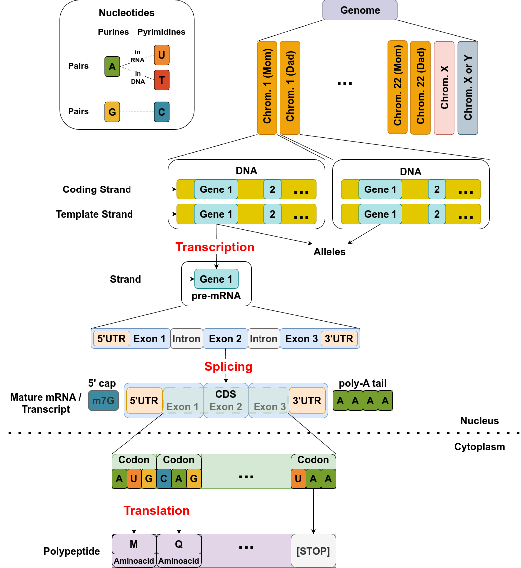
Source: Image by the author
It depicts a step-by-step overview of the central dogma of molecular biology: from DNA to functional protein. It starts with the genome, which consists of paired chromosomes inherited from each parent. Each chromosome contains genes, which are sequences of DNA. Genes have two strands: a coding strand and a template strand. During transcription, the template strand is used to synthesize a pre-mRNA molecule that includes untranslated regions (UTRs), exons, and introns.
Splicing removes the introns from the pre-mRNA and connects the exons to form mature mRNA. Additional modifications include the addition of a 5’ cap (m7G) and a 3’ poly-A tail, which are necessary for stability and export from the nucleus. In the cytoplasm, the mature mRNA is translated into a polypeptide chain. Ribosomes read codons—three-nucleotide sequences—in the coding sequence (CDS), matching them to amino acids to build a protein. Translation begins at a start codon (AUG) and ends at a stop codon, producing a functional polypeptide that will fold into a working protein.
Genome
The genome contains the complete set of genetic information for an organism. Amazingly, almost every cell in a multicellular organism carries its own full copy of the genome. In eukaryotes (animals, plants, fungi, seaweeds, and many unicellular organisms), the genome is housed in the cell nucleus. In contrast, prokaryotes (primarily bacteria and archaea) lack a nucleus, so their genetic material resides freely in the cytoplasm.
Genomics is the study of the structure, function, evolution, and analysis of an organism’s genome.
In humans, the genome (in most somatic cells, not reproductive cells) contains just over 6 billion base pairs, or roughly 12 billion nucleotides, unevenly distributed across 23 pairs of chromosomes.
Genome in Python
The Genome class below can be used to represent a genome and its chromosomes (we’ll define the Chromosome class in the next section).
class Genome(object):
    """
    Represents the complete genome of an organism, composed
    of a set of chromosomes.

    Attributes:
        chromosomes (list): A list of Chromosome objects
                            belonging to the organism.
        karyotype (int): The number of chromosomes in the
                         genome (including homologous pairs).
    """
    def __init__(self, chromosomes):
        self.chromosomes = chromosomes
        self.karyotype = len(chromosomes)

    def get_ith_chromosomes(self, i):
        """
        Retrieves all chromosomes with a given chromosome
        number (e.g., both homologous copies of chromosome 1).

        Parameters:
            i (int): Chromosome number to retrieve.

        Returns:
            list: Chromosome objects with the specified
                  chromosome number.
        """
        res = []
        for chrom in self.chromosomes:
            if chrom.number == i:
                res.append(chrom)
        return res

    def __repr__(self):
        """
        Returns a string representation of the genome by
        printing all chromosomes.
        """
        return '\n'.join([chrom.__repr__()
                          for chrom in self.chromosomes])
Chromosomes
The genome is organized into chromosomes — long DNA molecules. In prokaryotes, there’s typically a single circular chromosome. In eukaryotes, like humans, the genome is split across multiple linear chromosomes. Humans have 46 chromosomes, arranged in 23 pairs. One chromosome in each pair comes from your mother and the other from your father. When chromosomes are organized in pairs, the organism is said to be diploid; if only one set is present (as in gametes), it’s haploid. The two chromosomes in a pair are called homologous, meaning they carry the same genes in the same order, but not necessarily the same DNA sequence.
Each parent contributes a haploid set of 23 chromosomes — about 3 billion base pairs — to the child, resulting in a diploid genome of approximately 6 billion base pairs (or 12 billion nucleotides). However, this DNA isn’t evenly distributed across chromosomes, as shown in the illustration below:
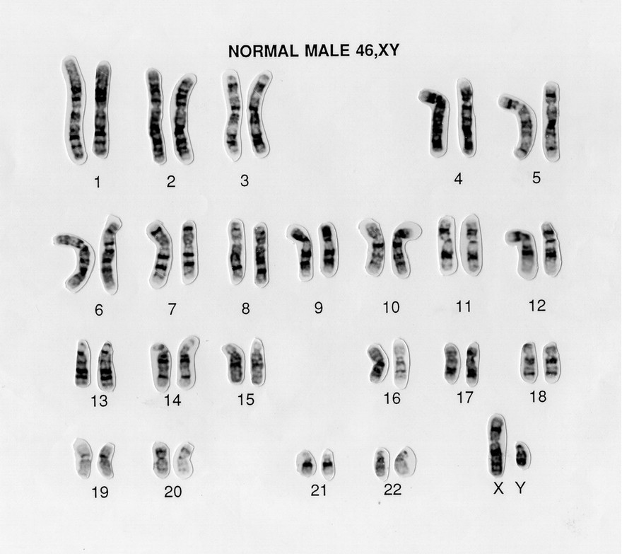
Source: Normal male 46,XY human karyotype. Wessex Reg. Genetics Centre. Wellcome Collection. Licensed under CC-BY 4.0
Human chromosomes vary greatly in size, ranging from about 47 million to 247 million base pairs. They’re numbered roughly in order of decreasing size, from chromosome 1 to 22. Interestingly, chromosome 21 is actually slightly shorter than chromosome 22. These 22 numbered chromosomes are called autosomes. The remaining two — X and Y — are known as sex chromosomes.
IMPORTANT: Although we inherit one chromosome of each pair from each parent, the sequences are remarkably similar. On average, the difference between homologous chromosomes is only about 0.2%. This means that out of 3 billion base pairs, about 2.994 billion are identical between maternal and paternal copies. Keep that in mind — it becomes especially important when we explore how DNA sequencing and variant analysis work (in another blog post).
The Human Genome Project
The Human Genome Project was a landmark scientific effort that, over 13 years, successfully mapped and sequenced the entire human genome, about 3 billion base pairs. This achievement resulted in the first version of a reference genome, a composite representation built by identifying consensus sequences (essentially, majority voting) across the genomes of multiple volunteers. Since the genomic difference between any two individuals is only about 0.2%, a shared reference could be reliably constructed.
With the reference genome in place, sequencing a new individual’s genome shifted from a de novo assembly (meaning, assembling it from scratch) challenge to a comparative one. This newer approach, called read alignment, involves mapping fragments of the individual’s DNA to corresponding regions in the reference genome, allowing for small mismatches that reflect individual variation.
(Not So) Fun Fact: An estimated 6%–8% of the human genome consists of sequences derived from endogenous retroviruses (ERVs)—ancient viruses that once integrated their genetic material into our ancestors’ DNA and have been inherited ever since.
(A Little) Fun Fact: Approximately 50% of the human genome consists of repeats, patterns that occur in multiple copies throughout the genome. One particularly abundant repeat is the Alu element, a short stretch of about 300 nucleotides that appears over 1 million times, accounting for roughly 10.7% of the entire genome.
Chromosome in Python
The Chromosome class below can be used to represent a chromosome, including its number, which parent it came from (0 or 1), if it’s an autosome or a sex chromosome, and its corresponding DNA (we’ll define the DNA class in the next section).
class Chromosome(object):
    """
    Represents a chromosome within a genome.

    Attributes:
        number (int): The chromosome number
                      (e.g., 1 for chromosome 1).
        homol_idx (int): Index identifying which homologous
                         chromosome it is (e.g., 0 or 1).
        dna (DNA): A DNA object representing the sequence
                   content of this chromosome.
        is_autosome (bool): Indicates whether the chromosome
                            is an autosome (True) or a sex
                            chromosome (False).
    """
    def __init__(self, number, homol_idx, dna,
                 is_autosome=True):
        # Chromosome number
        self.number = number
        # 0 or 1 to identify the homolog in a pair
        self.homol_idx = homol_idx
        # Autosomes are non-sex chromosomes
        self.is_autosome = is_autosome
        # Associated DNA sequence (double-stranded)
        self.dna = dna

    def __repr__(self):
        """
        Returns a brief string summary of the chromosome,
        including number, homolog index, and whether it's
        an autosome.
        """
        return f'chr #{self.number} | homologous \
            {self.homol_idx} | autosome {"T" \
            if self.is_autosome else "F"}'
DNA
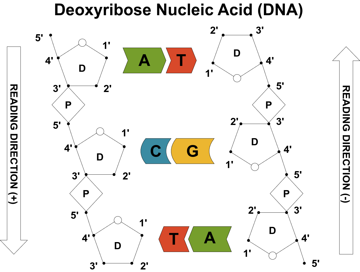
DNA, short for Deoxyribonucleic Acid, is a polymer composed of repeating units called nucleotides. Each DNA molecule consists of two long chains (or strands) coiled around each other to form the iconic double helix structure.
DNA has a well-defined structure. Each strand has a sugar-phosphate backbone, and the two strands are held together by specific base pairs: adenine (A) pairs with thymine (T), and cytosine (C) pairs with guanine (G). Because of this strict base-pairing, the two strands are complementary—knowing the sequence of one strand allows reconstruction of the other.
Despite strict base-pairing rules, the total amount of cytosine and guanine in a genome can differ significantly from the total amount of adenine and thymine. The proportion of guanine and cytosine is known as the GC-content, and it varies widely across species. In humans, the GC-content is about 42%, while in other organisms it ranges from as low as 20% in Plasmodium falciparum (the parasite responsible for malaria) to as high as 72% in the bacterium Streptomyces coelicolor.
Fun Fact: One full turn of the double helix spans about 10.5 base pairs (nucleotides per strand).
This complementarity is essential for DNA replication, which occurs during cell division (e.g., mitosis). Specialized enzymes like helicase first unzip the double helix by separating the two strands. Then DNA polymerase synthesizes new complementary strands by matching each exposed nucleotide with its pair. The result is two identical DNA molecules, each with one original strand and one newly synthesized strand.
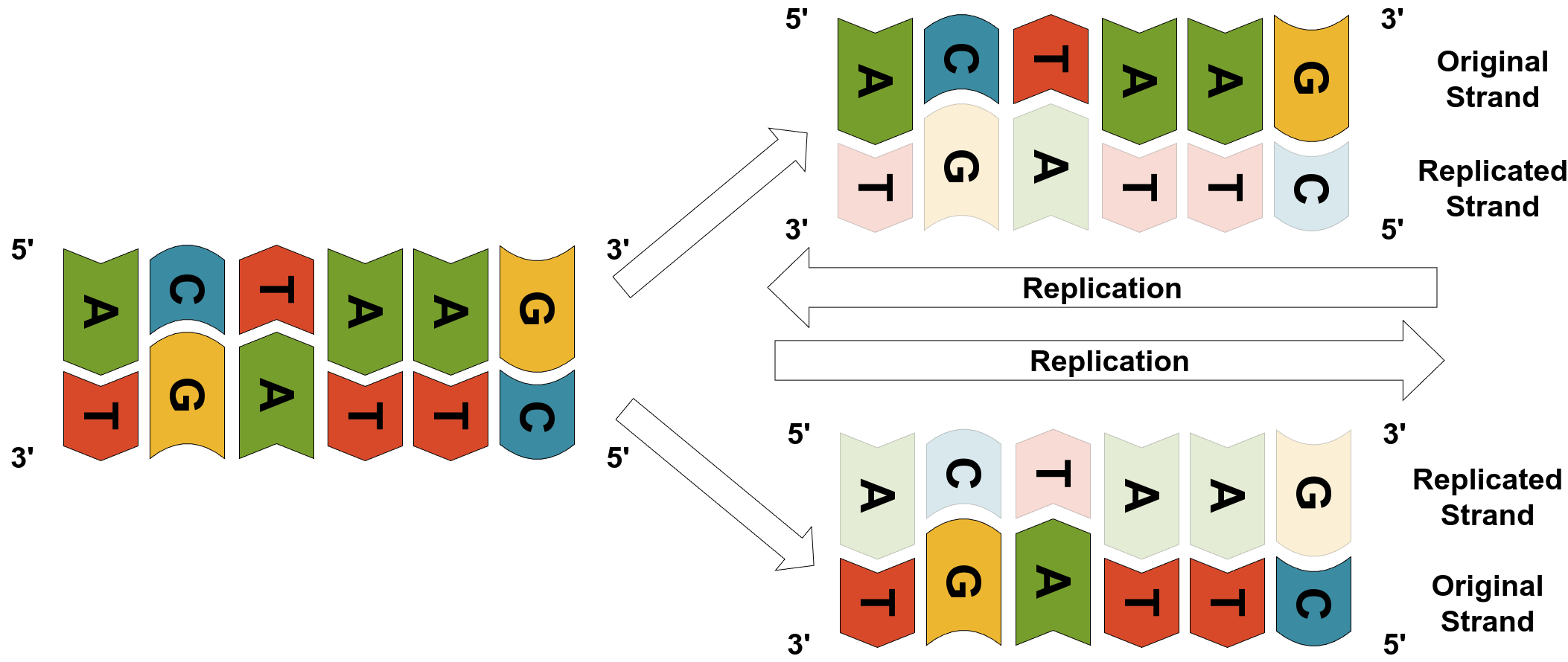
Source: Image by the author
Did you notice the 5’ and 3’ in the figure above? They indicate, respectively, the “head” and “tail” of each strand since new nucleotides can only be appended to the 3’ end of the strand. We’ll get back to it in a couple of sections.
Strand and DNA in Python
The DNA and Strand classes below can be used to represent a DNA molecule and its two component strands, each containing a sequence of nucleotides.
class DNA(object):
    """
    Represents a double-stranded DNA molecule.
    """
    def __init__(self, first_strand, second_strand):
        self.first_strand = first_strand
        self.second_strand = second_strand

class Strand(object):
    """
    Represents a DNA or RNA strand, storing its nucleotide
    sequence.

    Attributes:
        nucleotides (str): The sequence of nucleotide
                           bases (A, T, G, C, or U).
    """
    def __init__(self, nucleotides):
        self.nucleotides = nucleotides
DNA Replication in Python
The dna_polymerase() function can be used to synthesize a new complementary strand, and the replicate() function mimics the semi-conservative process of DNA replication.
def dna_polymerase(strand):
    """
    Simulates DNA replication by generating the complementary
    strand of a DNA sequence.

    Parameters:
        strand (Strand): The original strand to replicate.

    Returns:
        Strand: The complementary strand.
    """
    complement = str.maketrans("ATGC", "TACG")
    return Strand(strand.read().translate(complement))

def replicate(dna):
    """
    Simulates DNA replication by generating two identical
    DNA molecules from the original double-stranded DNA.

    Each strand of the original DNA serves as a template for
    the synthesis of a new complementary strand.

    Args:
        dna (DNA): The original DNA molecule to be replicated.

    Returns:
        tuple: A pair of new DNA objects representing the
               replicated molecules. Each consists of one
               original strand and one newly synthesized
               complementary strand.
    """
    # Use the original first strand as a template to create
    # its complement
    second_copy = dna_polymerase(dna.first_strand)

    # Use the original second strand as a template to create
    # its complement
    first_copy = dna_polymerase(dna.second_strand)

    # Return two new DNA molecules, each made from one
    # original and one new strand
    return (DNA(dna.first_strand, second_copy),
            DNA(first_copy, dna.second_strand))
Nucleotides
Nucleotides are the basic building blocks of DNA and RNA. In DNA, there are four types of nucleotides, each represented by a letter: A (adenine), C (cytosine), G (guanine), and T (thymine). RNA uses the same letters, except U (uracil) replaces T (thymine).
Nucleotides form specific base pairs through hydrogen bonding: A always pairs with T (or U in RNA), and C always pairs with G. That means if one strand has a C, the other must have a G at that position — never a T or A. These base pairs form the “rungs” of the DNA ladder.
Maybe the cartoon below can help you memorizing the pairs:
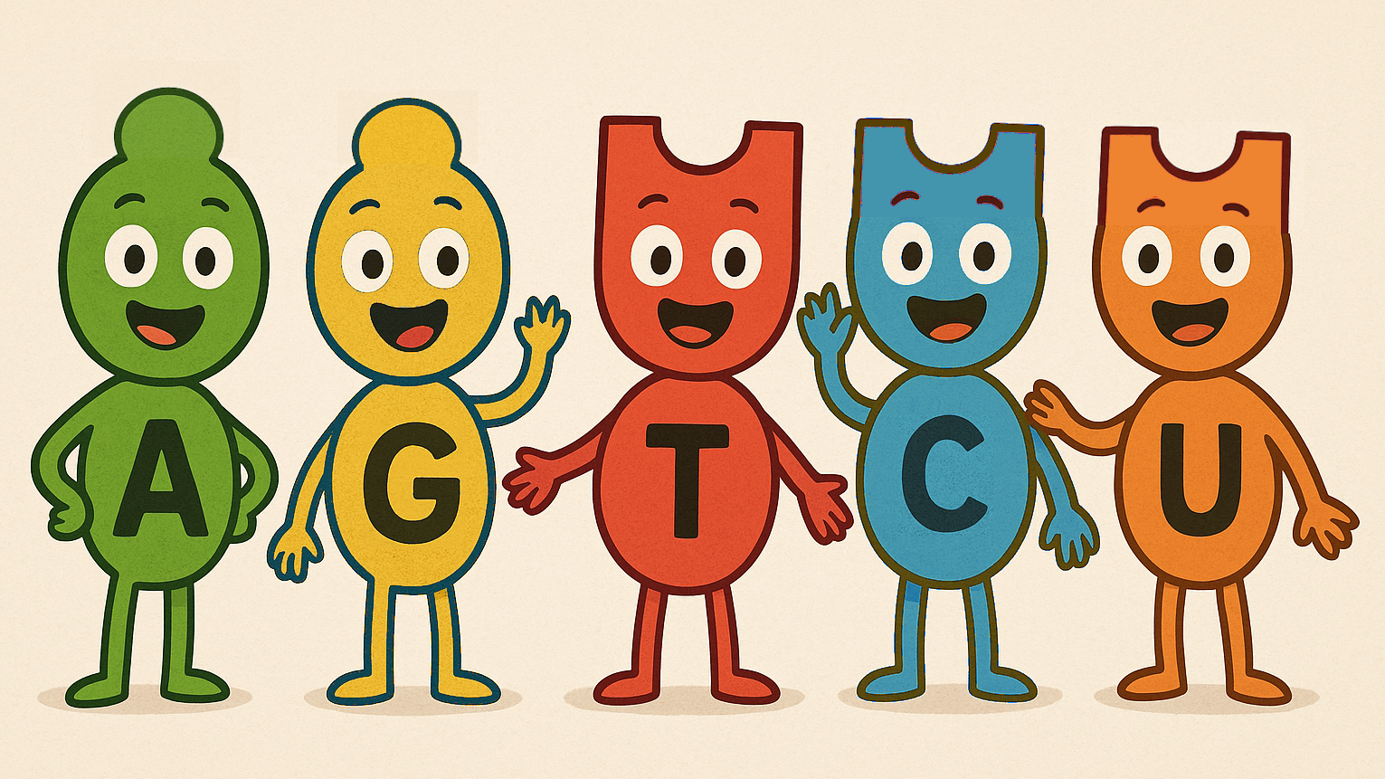
Source: Generated by the author
Did you notice that A and G have pointy heads while C, T, and U have dented heads? Chemically, nucleotides fall into two categories:
- Purines: double-ringed bases — adenine (A) and guanine (G)
- Pyrimidines: single-ringed bases — cytosine (C), thymine (T), and uracil (U)
Each nucleotide consists of a nitrogenous base (A, C, G, T, or U), a sugar (deoxyribose in DNA, ribose in RNA), and a phosphate group. In DNA, the sugars (D) and phosphates (P) link together in an alternating pattern to form the sugar-phosphate backbone — the “rails” of the DNA ladder. The bases stick out and pair across the two strands to form the ladder’s “rungs.”
Source: Image by the author
Deoxyribose and Strandness
The sugar in DNA — deoxyribose — gives DNA the “D” in its name. Deoxyribose is a five-carbon sugar with a ring-like structure, typically drawn as a pentagon. One corner of the ring contains an oxygen atom; the remaining four vertices are carbon atoms, numbered 1’ through 4’, starting to the right of the oxygen and proceeding clockwise. A fifth carbon (5’) is not part of the ring but branches off the 4’ carbon, as you can see in the figure below:
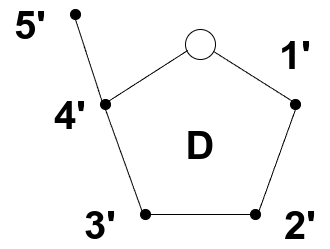
Source: Image by the author
Two of these carbon positions — 3’ and 5’ — play a critical structural role. They are the connection points for phosphate (P) groups that link nucleotides together in a chain. These connections define the directionality of a DNA strand. By convention, a DNA strand is read and written from the 5’ end (which has a free phosphate group) to the 3’ end (which has a free hydroxyl group). This is referred to as the 5’ to 3’ direction.
DNA is composed of two strands, and these strands are always aligned in opposite orientations — they are said to be anti-parallel. That means one strand runs from 5’ to 3’, while the other runs from 3’ to 5’. This directionality has major biological implications. For example, during DNA replication, new nucleotides can only be added to the 3’ end of a growing strand — a rule that governs how enzymes like DNA polymerase operate.
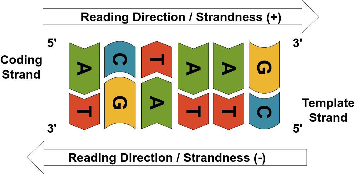
Source: Image by the author
Strand in Python (Improved)
We’re improving the Strand class to include strand direction.
class Strand(object):
    """
    Represents a DNA or RNA strand, storing its nucleotide
    sequence and directionality.

    Attributes:
        nucleotides (str): The sequence of nucleotide
                           bases (A, T, G, C, or U).
        is_positive (bool): Indicates the strand direction.
                            True for 5' to 3', False for
                            3' to 5'.
    """
    def __init__(self, nucleotides, is_positive=True):
        self.nucleotides = nucleotides
        self.is_positive = is_positive
        self.show_length = 80

    def __getitem__(self, index):
        # Supports slicing or indexing to return a new Strand
        # instance with the same orientation.
        return Strand(self.nucleotides[index],
                      self.is_positive)

    @property
    def positive(self):
        return self.is_positive

    def read(self):
        # Returns the raw nucleotide sequence.
        return self.nucleotides

    def show(self, length):
        # Defines the length of the nucleotide sequence shown
        self.show_length = length

    def __repr__(self):
        # Creates a readable representation showing
        # direction, sequence (trimmed if long),
        # and length.
        fprime = "(+) 5'"
        tprime = "(-) 3'"
        nucleotides = self.read()
        if len(nucleotides) > self.show_length:
            nucleotides = \
                nucleotides[:int(self.show_length/2)] + \
                '...' + \
                nucleotides[-int(self.show_length/2)+3:]
        return f'{fprime if self.is_positive else tprime} \
                 {nucleotides} {tprime[4:] \
                 if self.is_positive else fprime[4:]} \
                 ({len(self.read())} bps)'
DNA Replication in Python (Improved)
We’re also improving the dna_polymerase() function to account for strand direction.
def dna_polymerase(strand):
    """
    Simulates DNA replication by generating the complementary
    strand of a DNA sequence.

    Parameters:
        strand (Strand): The original strand to replicate.

    Returns:
        Strand: The complementary strand with reversed
                direction.
    """
    complement = str.maketrans("ATGC", "TACG")
    return Strand(strand.read().translate(complement),
                  not strand.positive)
Genes
You might assume the entire genome is made of genes — sections of DNA that actively encode biological instructions — but that’s far from the case. A gene is a region of DNA that contains the instructions for making a functional product, usually a protein. This process typically involves two steps: the gene is first transcribed into messenger RNA (mRNA), and then translated into a protein (we’ll unpack this later.)
Humans have around 21,000 protein-coding genes, yet these make up only about 2% of the total genome — roughly 60 million base pairs. The rest of the genome includes non-coding DNA, which contains regulatory elements, non-coding RNAs, introns (non-coding parts within genes, we’ll also get back to it later), repeat elements, and other sequences with varying or still-unknown functions.
Gene sizes vary widely. Some are just a few hundred base pairs long; others stretch over 2 million base pairs. The median human gene spans about 24,000 base pairs, though much of that may be non-coding intronic sequence.
Genes are distributed unevenly across chromosomes. For example, chromosome 1, the largest, contains around 2,800 genes, while chromosome 22, despite being the second-shortest, carries about 750 genes.
Gene in Python
The Gene class below can be used to define the region of a chromosome (in a given genome) corresponding to a particular gene.
class Gene(object):
    """
    Represents a gene located on a specific chromosome within
    a genome.

    Attributes:
        genome (Genome): The genome object this gene
                         belongs to.
        chr_number (int): The chromosome number where
                          the gene is located.
        start (int): The starting index (inclusive) of
                     the gene on the chromosome.
        end (int): The ending index (inclusive) of the
                   gene on the chromosome.
    """
    def __init__(self, genome, chr_number, start, end):
        self.genome = genome
        self.chr_number = chr_number
        self.start = start
        self.end = end

    def __repr__(self):
        """
        Provides a readable string representation of the
        gene location.
        """
        return f'Gene: chr #{self.chr_number} \
                 Position: {self.start}-{self.end}'
The Central Dogma of Molecular Biology
DNA’s role isn’t limited to making copies of itself. Its primary function is to store the genetic information needed to build the working molecules of life — especially proteins. But DNA doesn’t directly produce proteins. Instead, the process relies on an intermediary: RNA. This leads us to the Central Dogma of Molecular Biology, which describes the flow of genetic information within a cell.
The central dogma follows this path: DNA → RNA → Protein
- Transcription: A segment of DNA is used as a template to synthesize RNA. When this RNA carries instructions for making a protein, it’s called messenger RNA (mRNA).
- Translation: The mRNA is then decoded by ribosomes to assemble a protein, using the genetic code to translate nucleotide sequences into amino acid chains.
While not strictly part of the central dogma, DNA replication is also essential — it ensures that genetic information is preserved and passed on when cells divide.
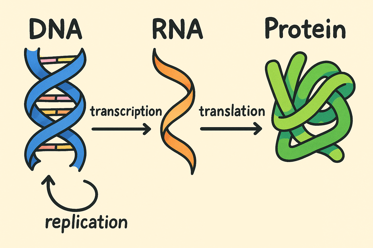
Source: Image generated by the author
RNA and Transcription
Ribonucleic acid (RNA) is a single-stranded molecule that acts as an intermediary in the process of gene expression. Specifically, messenger RNA (mRNA) serves as the template for assembling proteins. The process of creating mRNA from DNA is called transcription.
During transcription, one of the two DNA strands — called the template strand — is used to synthesize a complementary RNA molecule. The resulting RNA is nearly identical to the coding strand of the DNA, except that it uses uracil (U) instead of thymine (T).
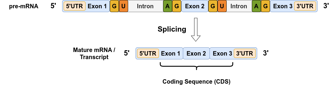
The initial product is called pre-mRNA (or precursor mRNA). It includes not just protein-coding sequences (called exons) but also non-coding segments called introns, as well as other untranslated regions (UTRs). Before the mRNA can be used to make a protein, it undergoes processing — including splicing, capping, and tailing — to produce a mature mRNA molecule that contains (almost) only the coding instructions.
![]()
Source: Image by the author
Key Difference: RNA uses the nucleotides A, C, G, and U (uracil), while DNA uses A, C, G, and T (thymine).
RNA and (Improved) DNA in Python
The RNA class below can be used to represent a single-strand mRNA molecule while indicating if it’s a precursor (pre-) mRNA or a mature mRNA. The improved DNA class makes a distinction between template and coding strands and includes a rich visual representation.
class RNA(object):
    """
    Represents an RNA molecule, either pre-mRNA or
    mature mRNA.

    Attributes:
        strand (Strand): The nucleotide sequence (as a
                         Strand object).
        is_pre (bool): Flag indicating whether the RNA is
                       pre-mRNA (True) or mature (False).
    """
    def __init__(self, strand, is_pre=True):
        self.strand = strand
        self.is_pre = is_pre

    def __repr__(self):
        """
        Returns a string representation of the RNA sequence.
        """
        # Get the basic string form from the strand object
        first = self.strand.__repr__()
        return f'RNA: {first}'


class DNA(object):
    """
    Represents a double-stranded DNA molecule with a
    positive (coding) and a negative (template) strand.
    """
    def __init__(self, first_strand, second_strand):
        assert first_strand.positive
        assert not second_strand.positive
        self.first_strand = first_strand
        self.second_strand = second_strand
        self.show_length = 80

    @property
    def template_strand(self):
        """Returns the negative (template) strand used in
        transcription."""
        return self.second_strand

    @property
    def coding_strand(self):
        """Returns the positive (coding) strand, identical
        to mRNA except T is used instead of U."""
        return self.first_strand

    def __getitem__(self, index):
        """
        Enables slicing of the DNA object, preserving both
        strands in the region.
        """
        return DNA(self.first_strand[index],
                   self.second_strand[index])

    def show(self, length):
        # Defines the length of the nucleotide sequence shown
        self.show_length = length
        self.first_strand.show(length)
        self.second_strand.show(length)

    def __repr__(self):
        """
        Visual representation of the DNA molecule showing
        base-pair alignment.
        """
        first = self.first_strand.__repr__()
        second = self.second_strand.__repr__()
        mid = ''.join(['|' if c in 'ATCGU' else ' '
                       for c in first])
        return f'DNA: {first}\n     {mid}\n     {second}'
Transcription in Python
The rna_polymerase() function below can be used to synthesize a new RNA strand in the transcription process. The transcribe() function takes an instance of DNA, the location of a particular gene, and applies the rna_polymerase() function to create the corresponding precursors mRNA.
def rna_polymerase(strand):
    """
    Simulates the action of RNA polymerase, transcribing a
    DNA strand into RNA.

    Args:
        strand (Strand): The DNA strand to be transcribed
                         (usually the template strand).

    Returns:
        Strand: The resulting RNA strand (complementary to
                the template strand).
    """
    # Transcription: A -> U, T -> A, G -> C, C -> G
    complement = str.maketrans("ATGC", "UACG")
    return Strand(strand.read().translate(complement),
                  not strand.positive)


def transcribe(dna, gene):
    """
    Transcribes the gene region from a DNA molecule into a
    pre-mRNA molecule.

    Args:
        dna (DNA): The full DNA molecule containing the gene.
        gene (Gene): The gene object, with start and end
                     indices on the chromosome.

    Returns:
        RNA: A pre-mRNA strand resulting from transcription
             of the gene.
    """
    start = gene.start
    end = gene.end
    # Extract the template strand segment corresponding
    # to the gene
    region = dna[start:end + 1].template_strand
    # Transcribe it into RNA
    return RNA(rna_polymerase(region), is_pre=True)
Gene Expression
A gene is said to be expressed when it is actively transcribed into RNA and, often, translated into protein. If the gene is not used — for regulatory or epigenetic reasons — it is considered silent or suppressed.
Gene expression levels can be quantified by measuring how much RNA is transcribed from that gene in a given sample. In practice, we count the number of RNA molecules that correspond to a gene using techniques like RNA sequencing (RNA-seq).
Gene expression is regulated by many factors, including transcription factors, chromatin structure, and environmental signals.
Alleles and Inheritance
Each gene exists in two copies in diploid organisms, one from each parent. These variants of a gene are called alleles. They occupy the same position (called a locus) on each homologous chromosome.
If both alleles are the same, either both “A” or both “a”, the individual is said to be homozygous for that gene. If the alleles differ (“A” and “a”) the individual is heterozygous.
In classical genetics, traits are often categorized as dominant or recessive:
- A dominant allele will determine the trait even if only one copy is present (e.g., Aa).
- A recessive allele only produces its associated trait when both copies are present (e.g., aa).
Note that dominance refers to phenotypic outcome, such as whether a pea appears green or yellow, not to the level of gene expression, meaning the number of RNA transcripts produced. A pea may display the yellow phenotype dictated by the dominant allele, even if that allele is expressed at a lower level than the recessive one.
Alleles in Python
The alleles() function below can be used to extract the two alleles/variants of a gene from a pair of homologous chromosomes.
def alleles(gene):
    """
    Extracts the two alleles (maternal and paternal variants)
    of a given gene from its chromosome pair in the genome.

    Args:
        gene (Gene): The gene object, which includes the
                     chromosome number and start/end
                     positions.

    Returns:
        tuple: A pair of DNA substrings representing the
               gene's alleles from the homologous
               chromosomes.
    """
    # Retrieve the homologous chromosome pair for the gene
    chrs = gene.genome.get_ith_chromosomes(gene.chr_number)

    # Determine consistent ordering based on homology index
    # (0 or 1)
    i = 0 if (chrs[0].homol_idx == 0) else 1

    # Slice the gene's sequence from both chromosomes
    return (
        chrs[i].dna[gene.start:gene.end + 1],
        chrs[1 - i].dna[gene.start:gene.end + 1]
    )
Exons and Introns
Genes make up only a small part of the genome — and surprisingly, not even all of a gene’s sequence is used directly to build proteins. The pre-mRNA produced during transcription is divided into alternating regions called exons and introns.
- Exons (expressed regions) contain the actual protein-coding instructions.
- Introns (intragenic regions) are non-coding segments that are located between exons; they are removed from the RNA transcript during a process called splicing.
At first glance, introns may seem wasteful, but they provide a key evolutionary benefit: they enable alternative splicing — the ability to produce multiple proteins from a single gene. By including or skipping different exons, the cell can create diverse protein products, called isoforms, from the same DNA sequence.
On average, mammalian genes contain 7–8 exons, but this number can vary widely. Exons are typically short (around 150 base pairs) while introns can range from hundreds to tens of thousands of base pairs. The first and last exons often include untranslated regions (UTRs) — parts of the RNA that are not translated into protein but play regulatory roles. After introns are spliced out, the resulting mature mRNA averages about 2,200 base pairs in length. The full set of protein-coding exons in the genome is called the exome, and it’s a major target in genetic and clinical research.
Splicing is driven by specific sequence motifs (i.e. patterns of nucleotide sequences) that mark the boundaries between exons and introns:
- Introns almost always start with a GT dinucleotide (in DNA; GU in RNA) and end with an AG.
- The 5’ splice site (exon-intron boundary) often matches consensus patterns like AG/GUAAGU or AG/GUCAGU, where GU (GT in the DNA strand) marks the start of the intron.
- The 3’ splice site (intron-exon boundary) typically ends with AG, preceded by variable patterns like UAG/ANNN, UAG/CNNN, GAG/ANNN, and GAG/CNNN (where N stands for any of the four bases), where AG marks the end of the intron.
While these motifs are not absolute rules, they guide the spliceosome, the cellular machinery that performs splicing. Exceptions exist, but most splicing events follow this general GT-AG rule.
Source: Image by the author
Exons and Introns in Python
The gt_ag_rule() function below can be used to identify the locations of introns in a gene for splicing. The find_introns() function below applies the gt_ag_rule() to the RNA and yields the intron sequences, in order. The get_exons() function removes the introns from the RNA and returns a sequence of exons, in order.
import re
import itertools

def gt_ag_rule(nucleotides, is_dna=True):
    """
    Identifies intron-like regions based on the GT/AG
    (or GU/AG) splicing rule.

    Args:
        nucleotides (str): The full nucleotide sequence.
        is_dna (bool): True if the sequence is DNA,
                       False if RNA.

    Returns:
        list: All matched intron sequences (non-greedy) that
              start with GT/GU and end with AG.
    """
    # In DNA, introns typically start with 'GT' and
    # end with 'AG'
    # In RNA, those become 'GU' and 'AG'
    pattern = r"(GT.*?AG)" if is_dna else r"(GU.*?AG)"
    intron_pattern = re.compile(pattern)
    return intron_pattern.findall(nucleotides)


def find_introns(rna):
    """
    Finds intron-like regions in an RNA sequence using
    the GU/AG rule.

    Args:
        rna (RNA): An RNA object.

    Returns:
        list: Intron-like subsequences based on the
              GU...AG pattern.
    """
    return gt_ag_rule(rna.strand.read(), is_dna=False)


def get_exons(rna, introns):
    """
    Splits the RNA sequence into exons by removing intron
    sequences.

    Args:
        rna (RNA): An RNA object.
        introns (list): A list of identified intron
                        subsequences.

    Returns:
        list: List of exon sequences (segments not matching
              any introns).
    """
    sequence = rna.strand.read()
    if not introns:
        # If no introns found, the entire strand is exon
        return [sequence]
    return re.split('|'.join(map(re.escape, introns)),
                    sequence)
Transcript (Mature mRNA)
After transcription, the pre-mRNA undergoes a series of processing steps: splicing (removal of introns), capping, and polyadenylation. The resulting single-stranded molecule is called a mature mRNA, or transcript.
You might assume that the entire mature mRNA is used to build a protein — but only part of it is. The actual coding sequence (CDS) contains the instructions for building a protein. Flanking the CDS are two non-coding sections: the 5’ untranslated region (5’ UTR) and the 3’ untranslated region (3’ UTR). These regions regulate gene expression, affecting things like mRNA stability, localization, and translation efficiency.
The complete set of RNA molecules in a cell is called the transcriptome, and the study of all transcripts is known as transcriptomics.
In eukaryotic cells, additional modifications are added:
- A 5’ cap (a modified guanine nucleotide) is attached to the beginning of the strand.
- A poly-A tail (a long string of adenosines, ~150–250 bases) is added to the end.
These features protect the mRNA from degradation, assist in export from the nucleus, and help the ribosome recognize the transcript during translation. Neither the cap nor the tail is directly encoded in the DNA, but a polyadenylation signal (typically AAUAAA or AUUAAA in RNA and AATAAA or ATTAAA in DNA) within the 3’ UTR triggers the addition of the tail.
IMPORTANT: Not every possible splice variant is viable. If a spliced mRNA lacks the poly-A signal or the cap, it won’t be exported from the nucleus or translated — it may be degraded instead.
Note: In our code examples, we use a shorter poly-A tail of just 10 A’s for simplicity, though real tails are much longer.
RNA in Python (Improved)
The RNA class below has an improved representation that includes capping and the poly-A tail.
class RNA(object):
    """
    Represents an RNA molecule, either pre-mRNA or
    mature mRNA.

    Attributes:
        strand (Strand): The nucleotide sequence
                         (as a Strand object).
        is_pre (bool): Flag indicating whether the RNA is
                       pre-mRNA (True) or mature (False).
        has_poly_a_tail (bool): Automatically derived from
                                is_pre; True if mature.
    """
    def __init__(self, strand, is_pre=True):
        self.strand = strand
        self.is_pre = is_pre
        # Mature RNAs have poly-A tails
        self.has_poly_a_tail = not is_pre
        self.show_length = 80

    def show(self, length):
        # Defines the length of the nucleotide sequence shown
        self.show_length = length
        self.strand.show(length-4-11*self.has_poly_a_tail)

    def __repr__(self):
        """
        Returns a string representation of the RNA sequence,
        with:
        - a 5' cap (m7G-) prepended
        - a 3' poly-A tail appended, if it's mature mRNA
        """
        # Get the basic string form from the strand object
        first = self.strand.__repr__()

        # Extract the raw nucleotide sequence from the
        # representation
        nucleotides = first.split(' ')[2]

        # Add 5' cap
        first = first.replace(nucleotides,
                              ' m7G-'+nucleotides)

        # Add 3' poly-A tail if it's a mature mRNA
        if self.has_poly_a_tail:
            first = first.replace(nucleotides,
                                  nucleotides+'-AAAAAAAAAA')

        return f'RNA: {first}'
RNA Splicing in Python
The splice() function below performs mRNA splicing, including alternative splicing, while making sure that only viable mRNA isoforms (those including both the cap and the poly-A tail) are flagged as mature.
def splice(rna):
    """
    Simulates alternative splicing of a pre-mRNA strand into
    multiple mRNA variants.

    This function generates all non-empty combinations of
    exons from the input pre-mRNA, checks each for a
    polyadenylation signal, and constructs mature or
    pre-mRNA variants accordingly.

    Parameters:
        rna: An instance of the RNA class.

    Returns:
        list of RNA: A list of RNA objects representing
                     different spliced variants. Each RNA
                     object is flagged as mature or pre-mRNA
                     depending on whether a polyadenylation
                     signal was found in the spliced
                     sequence.
    """
    # Identify intronic regions
    introns = find_introns(rna)
    # Extract exon sequences based on introns
    exons = get_exons(rna, introns)

    # Prepare all possible exon combinations
    exon_combinations = []
    for i in range(len(exons) + 1):
        exon_combinations.extend(
            itertools.combinations(exons, i)
        )

    # Store resulting mRNA variants
    spliced_variants = []
    # Skip empty combination (0)
    for combo in exon_combinations[1:]:
        # Concatenate selected exons into one sequence
        sequence = ''.join(combo)

        # Check for polyadenylation signal
        # (required for export & translation)
        signal_pos = (sequence.find('AAUAAA'),
                      sequence.find('AUUAAA'))
        valid_signals = [pos for pos in signal_pos if pos > 0]

        if valid_signals:
            # Mature mRNA: keep only up to and including
            # the signal
            signal_pos = min(valid_signals)
            strand = Strand(sequence[:signal_pos + 6])
            spliced_mrna = RNA(strand, is_pre=False)
        else:
            # Incomplete or non-exportable mRNA
            # (remains pre-mRNA)
            strand = Strand(sequence)
            spliced_mrna = RNA(strand, is_pre=True)

        spliced_variants.append(spliced_mrna)

    return spliced_variants
Codons and Coding Sequence (CDS)
The coding sequence (CDS) is the portion of a mature mRNA that gets translated into a protein. Each group of three bases is a codon, and each codon specifies a particular amino acid to be added to the growing protein chain. The CDS starts at a special codon (AUG), which not only marks the start of translation but also codes for the amino acid methionine (though it may be cleaved later).
Since the mRNA alphabet consists of four bases — A, C, G, and U — there are 4x4x4 = 64 possible codons, such as AAA, UGC, or CGA. Most codons code for an amino acid, but there are three special codons (UAA, UAG, and UGA) that act solely as stop signals to terminate the translation.
CDS and UTR in Python
The cds(), five_prime_utr(), and three_prime_utr() functions below can be used to divide the gene into their corresponding regions: coding sequence (CDS), 5’ untranslated region (UTR), and 3’ untranslated region (UTR). If a given region cannot be properly determined (e.g. lack of start codon), the function returns None.
def cds(rna):
    """
    Extracts the coding sequence (CDS) from a mature
    mRNA strand.

    This function scans the RNA sequence for a start codon
    (AUG), and reads triplets (codons) until a stop codon
    is encountered (UAA, UAG, UGA). The resulting coding
    sequence includes all codons from the start codon up to,
    but not including, the stop codon.

    Parameters:
        rna: An instance of the RNA class.

    Returns:
        str or None: The coding sequence as a string,
                     or None if no start codon is found.
    """
    # Read the full RNA strand sequence
    sequence = rna.strand.read()

    # Find the first occurrence of the start codon
    start_index = sequence.find("AUG")
    if start_index == -1:
        return None  # No start codon found, no CDS

    coding_sequence = ""

    # Process codons from start_index forward in triplets
    for i in range(start_index,
                   len(sequence) - len(sequence) % 3, 3):
        codon = sequence[i:i+3]
        coding_sequence += codon
        # Stop translation at stop codon
        if codon in ['UAA', 'UAG', 'UGA']:
            break

    return coding_sequence

def five_prime_utr(rna):
    """
    Extracts the 5' untranslated region (5' UTR) from
    a mature mRNA strand.

    This function prepends a 5' cap ("m7G-") to the RNA
    sequence, then returns all nucleotides from the
    beginning of the capped sequence up to (but not
    including) the start codon (AUG),  which marks the
    beginning of the coding sequence.

    Parameters:
        rna: An instance of the RNA class.

    Returns:
        str or None: The 5' UTR (including the cap) as
                     a string, or None if no start codon
                     is found.
    """
    # Read the full RNA strand sequence
    sequence = rna.strand.read()

    # Prepend the 5' cap
    sequence = 'm7G-' + sequence

    # Find the start codon to locate the beginning of the CDS
    start_index = sequence.find("AUG")
    if start_index == -1:
        return None  # No CDS found, so 5' UTR is undefined

    # Return everything before the start codon
    # (including the cap)
    return sequence[:start_index]

def three_prime_utr(rna):
    """
    Extracts the 3' untranslated region (3' UTR) from
    a mature mRNA strand.

    This function locates the first stop codon (UAA,
    UAG, or UGA) in the RNA sequence and returns the
    subsequence that follows it, including the poly-A
    tail if present. The 5' cap is prepended but not
    included in the returned UTR.

    Parameters:
        rna: An instance of the RNA class.

    Returns:
        str or None: The 3' UTR as a string (including the
                     poly-A tail if present), or None if
                     no stop codon is found.
    """
    # Read the RNA sequence
    sequence = rna.strand.read()

    # Prepend the 5' cap (not used for 3' UTR, but
    # consistent with other operations)
    sequence = 'm7G-' + sequence

    # Append the poly-A tail if present
    if rna.has_poly_a_tail:
        sequence += '-AAAAAAAAAA'  # simplified poly-A tail

    # Locate all stop codon positions (skip if not found)
    stop_positions = (sequence.find('UAA'),
                      sequence.find('UAG'),
                      sequence.find('UGA'))
    valid_stops = [pos for pos in stop_positions if pos > 0]

    if not valid_stops:
        return None  # No valid stop codon found

    # Select the first occurring stop codon
    stop_index = min(valid_stops)

    # Return sequence after the stop codon (i.e., the 3' UTR)
    return sequence[stop_index + 3:]
Amino Acids and Translation
Once the mature mRNA is exported from the nucleus into the cytoplasm, it is picked up by a ribosome — a molecular machine that reads the RNA three nucleotides (one codon) at a time.
Although there are 64 possible codons, the genetic code is degenerate or redundant, meaning multiple codons can specify the same amino acid. For example, the codons GCU, GCC, GCG, and GCA all code for alanine. This redundancy helps buffer against some mutations.
Translation begins at a specific start codon, which has the nucleotide sequence AUG, and ends at one of the stop codons (UAA, UAG, or UGA). Once the ribosome encounters one of these stop codons, it halts translation, releasing the completed protein. All codons between the start codon and the stop codon are translated in order, one at a time, into a chain of amino acids — a polypeptide — which folds into a functional protein.
To determine which amino acid a codon corresponds to, a codon wheel (shown below) can be used. You start from the center of the wheel and move outward: the amino acid name or abbreviation appears in the outermost layer.
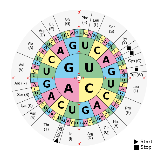
Source: Wikipedia, image released into the public domain by its author, Mouagip
Translation in Python
The codon_table dictionary below can be used to translate codons into amino acids. The translate() function below can be used to effectively translate an instance of mRNA into its corresponding polypeptide chain. If no coding sequence is found in the mRNA, the function returns “non-coding RNA.”
codon_table = {
    "AUG": "M",
    "AUA": "I", "AUC": "I", "AUU": "I",
    "AGG": "R", "AGA": "R",
    "AGC": "S", "AGU": "S",
    "AAG": "K", "AAA": "K",
    "AAC": "N", "AAU": "N",
    "ACG": "T", "ACA": "T", "ACC": "T", "ACU": "T",
    "CGG": "R", "CGA": "R", "CGC": "R", "CGU": "R",
    "CAG": "Q", "CAA": "Q",
    "CAC": "H", "CAU": "H",
    "CCG": "P", "CCA": "P", "CCC": "P", "CCU": "P",
    "CUG": "L", "CUA": "L", "CUC": "L", "CUU": "L",
    "UGG": "W",
    "UGC": "C", "UGU": "C",
    "UAC": "Y", "UAU": "Y",
    "UCG": "S", "UCA": "S", "UCC": "S", "UCU": "S",
    "UUG": "L", "UUA": "L",
    "UUC": "F", "UUU": "F",
    "GGG": "G", "GGA": "G", "GGC": "G", "GGU": "G",
    "GAG": "E", "GAA": "E",
    "GAC": "D", "GAU": "D",
    "GCG": "A", "GCA": "A", "GCC": "A", "GCU": "A",
    "GUG": "V", "GUA": "V", "GUC": "V", "GUU": "V",
    "UAA": "STOP", "UAG": "STOP", "UGA": "STOP"
}

def translate(rna):
    """
    Translates a mature mRNA sequence into a polypeptide
    chain.

    This function extracts the coding sequence (CDS) from
    the given RNA strand and translates it into a sequence
    of amino acids using the codon table. If the RNA does
    not contain a valid CDS (e.g., missing start codon or
    stop codon), the function returns 'non-coding RNA'.

    Parameters:
        rna: An instance of the RNA class.

    Returns:
        str: A polypeptide (amino acid sequence),
             or 'non-coding RNA' if no valid CDS is found.
    """
    polypeptide = ""

    # Extract the coding sequence from the RNA
    sequence = cds(rna)

    # Return early if no valid coding sequence is found
    if sequence is None:
        return 'non-coding RNA'

    # Iterate over the CDS in codons
    # (groups of 3 nucleotides)
    for i in range(0, len(sequence), 3):
        codon = sequence[i:i+3]

        # Look up the amino acid for this codon
        amino_acid = codon_table[codon]

        # Stop translation at stop codon;
        # do not include it in the output
        if amino_acid != "STOP":
            polypeptide += amino_acid

    return polypeptide
Proteins
A chain of amino acids produced by the ribosome is called a polypeptide. A protein consists of one or more polypeptide chains that fold into a specific 3D structure and work together as a functional unit.
After translation, polypeptides often undergo post-translational modifications that affect their folding, stability, localization, activity, and overall function.
Proteomics is the large-scale study of proteins — including their structures, functions, modifications, and interactions.
Although gene expression, often measured by quantifying mRNA molecules in a sample, can serve as a proxy for protein production, the relationship is not always straightforward. mRNA transcripts vary in stability; some degrade quickly after being translated only a few times, while others persist and are translated repeatedly. In addition, protein molecules themselves have widely different half-lives, ranging from hours to over a week, further influencing the correlation between mRNA abundance and protein levels.
Example
Let’s work through an example using a hypothetical diploid eukaryotic organism that has a single chromosome containing a single gene.
First, we create the genetic material of its mother: starting from a coding strand of DNA, we apply DNA polymerase to generate the complementary template strand. There we have it—our first piece of double-stranded DNA.
coding_strand_0 = Strand('TGCGATCGAACGGACCATGGCAAGAAAGGTTCATTGCGGACAGACCTGGGCAATTAACGTCCAACCACAGTGGGCTTCGGTTTTAACGCGGCAGCACGAGCGTGAATAATTCGCAATAAACGATTACA')
template_strand_0 = dna_polymerase(coding_strand_0)
dna_0 = DNA(coding_strand_0, template_strand_0)
dna_0.show(50)
dna_0
Output
DNA: (+) 5' TGCGATCGAACGGACCATGGCAAGA...TAATTCGCAATAAACGATTACA 3' (128 bps)
            |||||||||||||||||||||||||   ||||||||||||||||||||||
     (-) 3' ACGCTAGCTTGCCTGGTACCGTTCT...ATTAAGCGTTATTTGCTAATGT 5' (128 bps)
Next, we do the same to create the genetic material of its father.
coding_strand_1 = Strand('TGCGATCGAACGGACCATGGCAAGAAAGGTTCATTGCGGACAGACCTGGGCAATTAACGTCCAACCACAGTGGGCTTCGGTTTTACCGCAGACGCACGAGCGTGAATAATTCGCAATAAACGATTACA')
template_strand_1 = dna_polymerase(coding_strand_1)
dna_1 = DNA(coding_strand_1, template_strand_1)
dna_1.show(50)
dna_1
Output
DNA: (+) 5' TGCGATCGAACGGACCATGGCAAGA...TAATTCGCAATAAACGATTACA 3' (128 bps)
            |||||||||||||||||||||||||   ||||||||||||||||||||||
     (-) 3' ACGCTAGCTTGCCTGGTACCGTTCT...ATTAAGCGTTATTTGCTAATGT 5' (128 bps)
One chromosome from the mother, another from the father, we have our little genome ready:
chr1_0 = Chromosome(1, 0, dna_0, is_autosome=True)
chr1_1 = Chromosome(1, 1, dna_1, is_autosome=True)
genome = Genome([chr1_0, chr1_1])
genome
Output
chr #1 | homologous 0 | autosome T
chr #1 | homologous 1 | autosome T
This particular organism has a single gene on its chromosome: the MT gene (you’ll soon see why it’s called MT). The gene spans positions 10 to 122 on the chromosome (in reality, the location of a gene within a chromosome varies and it is determined during the read alignment process).
mt_gene = Gene(genome, 1, 10, 122)
mt_gene
Output
Gene: chr #1 Position: 10-122
Let’s check the alleles—the two different versions of the gene in each chromosome of the pair:
mt_alleles = alleles(mt_gene)
mt_alleles[0].show(40)
mt_alleles[1].show(40)
mt_alleles
Output
(DNA: (+) 5' CGGACCATGGCAAGAAAGGT...TAATTCGCAATAAACGA 3' (113 bps)
             ||||||||||||||||||||   |||||||||||||||||
      (-) 3' GCCTGGTACCGTTCTTTCCA...ATTAAGCGTTATTTGCT 5' (113 bps),
 DNA: (+) 5' CGGACCATGGCAAGAAAGGT...TAATTCGCAATAAACGA 3' (113 bps)
             ||||||||||||||||||||   |||||||||||||||||
      (-) 3' GCCTGGTACCGTTCTTTCCA...ATTAAGCGTTATTTGCT 5' (113 bps))
We can’t really tell but the two alleles are slightly different from one another. We’ll transcribe and translate the first one (from chr1_0) and you’ll try your hand with the other one (chr1_1) to find the difference in translation.
Now, let’s transcribe the gene from the first chromosome:
rna = transcribe(chr1_0.dna, mt_gene)
rna.show(40)
rna
Output
RNA: (+) 5' m7G-CGGACCAUGGCAAGAAAG...AUUCGCAAUAAACGA 3' (113 bps)
Notice the “m7G” cap prepended to the RNA strand. It’s one of the modifications mRNA undergoes to allow export from the nucleus to the cytoplasm.
It’s time to splice the pre-mRNA. First, let’s identify the introns:
introns = find_introns(rna)
introns
Output
['GUUCAUUGCGGACAG', 'GUCCAACCACAG', 'GUUUUAACGCGGCAG']
What about the exons?
exons = get_exons(rna, introns)
exons
Output
['CGGACCAUGGCAAGAAAG',
 'ACCUGGGCAAUUAAC',
 'UGGGCUUCG',
 'CACGAGCGUGAAUAAUUCGCAAUAAACGA']
Remember, splicing allows for different combinations of exons, as long as their ordering is preserved:
transcripts = splice(rna)
transcripts
Output
[RNA: (+) 5'  m7G-CGGACCAUGGCAAGAAAG 3' (18 bps),
 RNA: (+) 5'  m7G-ACCUGGGCAAUUAAC 3' (15 bps),
 RNA: (+) 5'  m7G-UGGGCUUCG 3' (9 bps),
 RNA: (+) 5'  m7G-CACGAGCGUGAAUAAUUCGCAAUAAA-AAAAAAAAAA 3' (26 bps),
 RNA: (+) 5'  m7G-CGGACCAUGGCAAGAAAGACCUGGGCAAUUAAC 3' (33 bps),
 RNA: (+) 5'  m7G-CGGACCAUGGCAAGAAAGUGGGCUUCG 3' (27 bps),
 RNA: (+) 5'  m7G-CGGACCAUGGCAAGAAAGCACGAGCGUGAAUAAUUCGCAAUAAA-AAAAAAAAAA 3' (44 bps),
 RNA: (+) 5'  m7G-ACCUGGGCAAUUAACUGGGCUUCG 3' (24 bps),
 RNA: (+) 5'  m7G-ACCUGGGCAAUUAACCACGAGCGUGAAUAAUUCGCAAUAAA-AAAAAAAAAA 3' (41 bps),
 RNA: (+) 5'  m7G-UGGGCUUCGCACGAGCGUGAAUAAUUCGCAAUAAA-AAAAAAAAAA 3' (35 bps),
 RNA: (+) 5'  m7G-CGGACCAUGGCAAGAAAGACCUGGGCAAUUAACUGGGCUUCG 3' (42 bps),
 RNA: (+) 5'  m7G-CGGACCAUGGCAAGAAAGACCUGGGCAAUUAACCACGAGCGUGAAUAAUUCGCAAUAAA-AAAAAAAAAA 3' (59 bps),
 RNA: (+) 5'  m7G-CGGACCAUGGCAAGAAAGUGGGCUUCGCACGAGCGUGAAUAAUUCGCAAUAAA-AAAAAAAAAA 3' (53 bps),
 RNA: (+) 5'  m7G-ACCUGGGCAAUUAACUGGGCUUCGCACGAGCGUGAAUAAUUCGCAAUAAA-AAAAAAAAAA 3' (50 bps),
 RNA: (+) 5'  m7G-CGGACCAUGGCAAGAAAGACCUGGGCAAUUAACUGGGCUUCGCACGAGCGUGAAUAAUUCGCAAUAAA-AAAAAAAAAA 3' (68 bps)]
Out of the 15 theoretical isoforms, did you notice anything in particular?
Some have poly-A tails, some do not. Those mRNAs without a poly-A tail will be degraded, so we ignore them.
transcripts_with_tails = [t for t in transcripts if t.has_poly_a_tail]
transcripts_with_tails
Output
[RNA: (+) 5'  m7G-CACGAGCGUGAAUAAUUCGCAAUAAA-AAAAAAAAAA 3' (26 bps),
 RNA: (+) 5'  m7G-CGGACCAUGGCAAGAAAGCACGAGCGUGAAUAAUUCGCAAUAAA-AAAAAAAAAA 3' (44 bps),
 RNA: (+) 5'  m7G-ACCUGGGCAAUUAACCACGAGCGUGAAUAAUUCGCAAUAAA-AAAAAAAAAA 3' (41 bps),
 RNA: (+) 5'  m7G-UGGGCUUCGCACGAGCGUGAAUAAUUCGCAAUAAA-AAAAAAAAAA 3' (35 bps),
 RNA: (+) 5'  m7G-CGGACCAUGGCAAGAAAGACCUGGGCAAUUAACCACGAGCGUGAAUAAUUCGCAAUAAA-AAAAAAAAAA 3' (59 bps),
 RNA: (+) 5'  m7G-CGGACCAUGGCAAGAAAGUGGGCUUCGCACGAGCGUGAAUAAUUCGCAAUAAA-AAAAAAAAAA 3' (53 bps),
 RNA: (+) 5'  m7G-ACCUGGGCAAUUAACUGGGCUUCGCACGAGCGUGAAUAAUUCGCAAUAAA-AAAAAAAAAA 3' (50 bps),
 RNA: (+) 5'  m7G-CGGACCAUGGCAAGAAAGACCUGGGCAAUUAACUGGGCUUCGCACGAGCGUGAAUAAUUCGCAAUAAA-AAAAAAAAAA 3' (68 bps)]
We’re left with 8 isoforms. Still, not all of them contain a well-defined coding sequence (CDS)—some may lack a start codon (AUG). Let’s filter those out too:
transcripts_with_cds = [t for t in transcripts_with_tails if cds(t) is not None]
transcripts_with_cds
Output
[RNA: (+) 5'  m7G-CGGACCAUGGCAAGAAAGCACGAGCGUGAAUAAUUCGCAAUAAA-AAAAAAAAAA 3' (44 bps),
 RNA: (+) 5'  m7G-CGGACCAUGGCAAGAAAGACCUGGGCAAUUAACCACGAGCGUGAAUAAUUCGCAAUAAA-AAAAAAAAAA 3' (59 bps),
 RNA: (+) 5'  m7G-CGGACCAUGGCAAGAAAGUGGGCUUCGCACGAGCGUGAAUAAUUCGCAAUAAA-AAAAAAAAAA 3' (53 bps),
 RNA: (+) 5'  m7G-CGGACCAUGGCAAGAAAGACCUGGGCAAUUAACUGGGCUUCGCACGAGCGUGAAUAAUUCGCAAUAAA-AAAAAAAAAA 3' (68 bps)]
We can now inspect the three regions of one of the valid transcripts: CDS, 5’ UTR, and 3’ UTR.
cds(transcripts_with_cds[0]), five_prime_utr(transcripts_with_cds[0]), three_prime_utr(transcripts_with_cds[0])
Output
('AUGGCAAGAAAGCACGAGCGUGAAUAA', 'm7G-CGGACC', 'AUAAUUCGCAAUAAA-AAAAAAAAAA')
The CDS starts with an AUG codon and ends with an UAA stop codon, which is not translated. The 5’ UTR includes the cap and a few nucleotides before the CDS. The 3’ UTR contains the polyadenylation signal (AAUAAA) and the poly-A tail.
Finally, we translate the four viable mRNAs into polypeptide chains:
polypeptides = [translate(t) for t in transcripts_with_cds]
polypeptides
Output
['MARKHERE', 'MARKTWAINHERE', 'MARKWASHERE', 'MARKTWAINWASHERE']
Now you know why it’s called the MT (Mark Twain) gene. 🙂
Try transcribing the MT gene from the other chromosome (chr1_1) and see what you get.
Have fun!